Lab: Using Data

Introduction

The purpose of this mini-lab is to practice loading data, plotting data, saving figures, and fitting data to a model.

Loading Data into an Array

Create a new file for the statements and functions you will write in this mini-lab. Save this new file with a name representative of this mini-lab.
It is often useful for us to plot an array of data that we either generate from our own code, or that we read in from a file. Download the file class-grades.csv and save it in the same folder as this lab file. This data set is a set of grades from a Chemical Engineering course at MacMaster University. This data set contains 99 rows and six columns. The columns give us: a prefix denoting which year the student is, the assignment grade, the tutorial grade, the midterm grade, the takehome exam grade, and the final exam grade for each student. The following code may be used to read this data into an array of size 99x6:
```
    def readGrades():
        gradeArray = np.zeros((99,6)) 
        with open('class-grades.csv', 'r') as f:
            
            # read from the file, a line at time, adding it to a list
            index = 0
            for grades in csv.reader(f):
                gradeArray[index] = [float(grades[0]), float(grades[1]), float(grades[2]), float(grades[3]), float(grades[4]), float(grades[5])]
                index += 1
        
        print(gradeArray)
    
```
Copy this code and test it to see what it does. Notice that the rows in the array correspond to the rows of the data file.
NumPy has a function, loadtxt that will do this same thing for us, where we don't have to read the data line by line, put it into the list, and then convert the list to an array. Our new statement would look like:
```
gradeSet = np.loadtxt('class-grades.csv', delimiter = ',')
```
(Note: the delimiter is used to specify what separates the items on each line of the data file. Since our data is in a .csv (Comma Separated Values) file, we use a comma. ) Copy this statement and print out the array.
One question we can ask about this data is how many homework grades fall into different categories. To create a histogram of homework grades, try the following:
```
    hwGrades = [gradeArray[i][1] for i in range(len(gradeArray))]
    plt.hist(hwGrades, 20)
    
```
(Remember, you will need to import matplotlib.pyplot in order to use the hist function.)
Create a histogram of the final exam scores.
The file JanTemps.csv contains the daily high and low temps for the month of January, for each of the years 1980, 2005, 2010, 2020, and 2021. This is the same data that was used in Lab 3: Using Arrays. Download this csv file and read the data into a 31x10 array. Print this array.
Create a histogram for one set of temperatures (either the high temps or low temps for one year).
Plot all 5 sets of high temps in the same figure and all 5 sets of low temps in the same figure. Do you see any patterns?

Saving Figures

In the previous set of exercises, you created a histogram showing the distribution of the homework grades for the 99 students. When you end your session in Spyder (or whatever development environment you are using), your figures will disppear. If you wrote a script (i.e, code) to create this histogram, you can always recreate the figure. It is possible you would like to use this figure (or another one) in a report of some kind. Saving figures is straightfoward.

If your figure pops up in a separate window, click on the icon at he bottom that looks like a diskette. Then give the figure an appropriate name, and choose which format you would like to save it in. Pyplot will create a graphics file of the type you requested.
To save a figure from the iPython command prompt, or from within a script, use the plt.savefig command. For example,
```
plt.savefig("hwGrades.png")
```
The plot will be saved in your current working directory.
Save one of your temperature plots.

CHALLENGE EXERCISES (Optional) Fitting HIV Data to a Model^*

A viral load is the number of virions in the blood of a patient infected with HIV after the administration of an antiretroviral drug. One model for the viral load predicts that the concentration V(t) of HIV in the blood at time t after the start of treatment will be

V(t) = Aexp(-αt) + Bexp(-βt).

The four parameters A, α, B, and β are constants that control the behavior of the model.
In this section, we will use Python to generate plots based on this model, import and plot experimental data, and then fit model parameters to the data⁺.

Create an array of 101 numbers ranging from 0 to 10 using the linspace function. Assign it to the variable time.
Create variables named A, alpha, B, and beta, and give them some initial values. You might start with B as 0 to get an idea of how the function V(t) will work.
Next, create an array called viralLoad of viral load values corresponding to the time values. (Remember, if nums is an array of 10 numbers, to multiply and add something to each of these array values, we could type a statement like newNums = 3 * nums + 7.)
You now have two arrays of the same length, so plot them, as in
```
plt.plot(time, viralLoad).
```
Remember that to see just the points, you can specify a color and shape to be used for the points, such as
```
plt.plot(time, viralLoad,'ro').
```
Label the axes of your graph "Time" (x-axis) and "Viral Load" (y-axis).
Experiment with different values of A, alpha, B, and beta to see how the shape of the graph changes.
Download the file HIVseries.csv, which contains experimental HIV data. Use the np.loadtxt command to load the data into an array called HIV_Data.
Create an array called time from the first column of the HIV_Data array.
Create an array called viralLoad from the second column of the HIV_Data array.
Plot these time and viral load arrays the same way you plotted the previous time and viralLoad arrays.
Create a new array, called viralLoadFcnArray by computing the values of the viral load function for this new time array. (Create it the same way as you first created the viral load array, by using the function for viral load.)
Plot this new array on the same axis with the experimental data. Plot this function as a curve, and use just the points for the experimental data. You might end up with something such as:
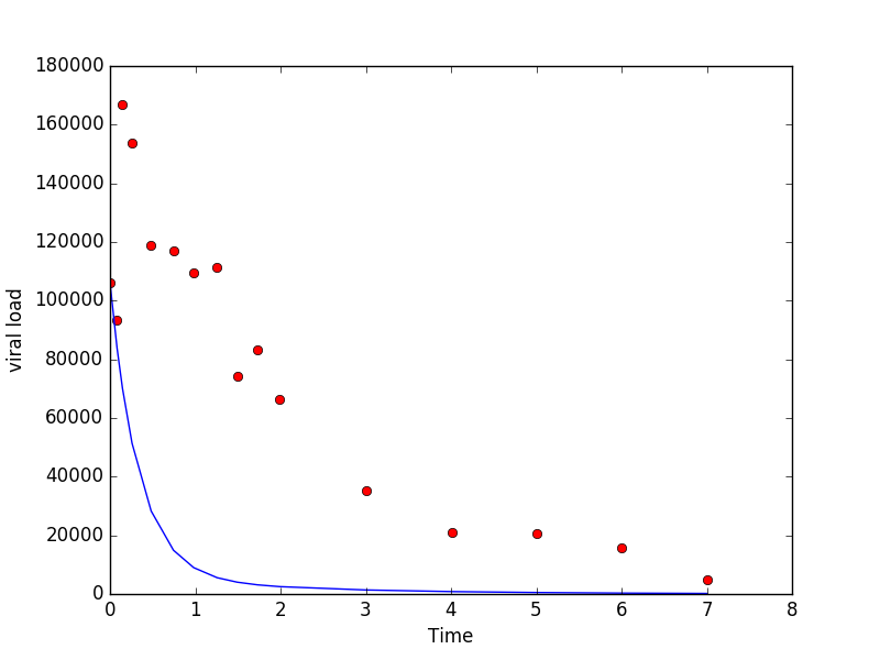
The goal now is to tune the four parameters of the viral load function until the model agrees with the data. It is hard to find the right needle in a 4-dimensional haystack! So let's try to be a little more systematic about it. Think about how the initial value V(0) depends on the four constants. What does it tell us about A and B? Now vary your constants (assuming β > α) so that you always get the correct initial value. Next experiment with α and β so that your long term behavior matches that of the data. Continue adjusting the four parameters until you are satisfied that your model is now a good fit for the data.

^*This example is taken from Kinder, J.and Nelson, P., "A Student's Guide to Python for Physical Modeling", Princeton University Press, 2015, pp. 61 - 63.
⁺For more details of this model, see Chapter 1 of Nelson, "Physical Models of Living Systems", W.H. Freeman, 2015.

Submit

When you are satisfied your code is working properly, update the description of the program in the comments at the top of your file, add comments to your code to describe what you are doing, and then submit the file you created for this lab, along with one of the figures you saved, via Kit.